Introduction

Imbalanced data typically refers to a model with classification problems where the classes are not represented equally(e.g. 90% of the data belongs to one class). They are commonly seen in fraud detection, cancer detection, manufacturing defects, and online ads conversion analytics.

Working on an imbalanced dataset tends to be extremely tricky as simple classification algorithms tend to struggle in such situations, usually resulting in overfitting on the majority class and completely ignoring the minority class. This post details a guide on how to conduct data analysis and machine learning using an imbalanced dataset to predict a classification outcome.

The dataset in this project is taken from the UCI Machine Learning Repository. However you will find the column names not included in the dataset- you can download the training data and the test data in the links below, courtesy of the Analytics Vidhya team:

Download Training Data

Download Test data

1. The Problem Statement

“Given various features, the aim is to build a predictive model to determine the income level for people in US. The income levels are binned at below 50K and above 50K.”

From the problem statement, it’s evident that this is a binary classification problem, to find out if the income level is below or above 50k, based on a set of features stated below:

1. Age
2. Marital Status
3. Income
4. Family Members
5. No. of Dependents
6. Tax Paid
7. Investment (Mutual Fund, Stock)
8. Return from Investments
9. Education
10. Spouse Education
11. Nationality
12. Occupation
13. Region in US
14. Race
15. Occupation category

Note: I will be completing the data exploration / data manipulation using Python and the machine learning portion using R.

2. Data Exploration

Let’s begin by importing the libraries required, and loading the training data and test data into Python.

#Importing the libraries
import pandas as pd
import numpy as np
import matplotlib.pyplot as plt
#To display our plots and graphs inline
%matplotlib inline

#Loading the train and test data
train = pd.read_csv("C:/Users/ML/Documents/train.csv")
test = pd.read_csv("C:/Users/ML/Documents/test.csv")

#how many columns our training dataset has
train.info()

<class 'pandas.core.frame.DataFrame'>
RangeIndex: 199523 entries, 0 to 199522
Data columns (total 41 columns):
.
.

#how many rows our training dataset has
len(train)

199523

#how many rows our training dataset has
len(test)

99762

We see that train data has 199523 rows & 41 columns, and test data has 99762 rows and 41 columns. Generally, test data comes with one less column than train (the variable we want to predict; income_level). It means that this data set has test prediction values also. This will help us in evaluating our model.

Let’s verify the target variable we want to predict for both train and test datasets.

train['income_level'].value_counts()

-50000 187141
50000 12382
Name: income_level, dtype: int64

test['income_level'].value_counts()

-50000 93576
50000+. 6186
Name: income_level, dtype: int64

We can already see some discrepancy in our target variable- the value 50000 is different across train and test data. This disparity will cause trouble in model evaluation. Being a binary classification problem, we can encode these variables as 0 and 1. I’m showing two different ways(for train and test data) we can do this below.

#Changing train dataset income levels to binary
train['income_level'].replace(-50000, '0',inplace=True)
train['income_level'].replace(50000, '1',inplace=True)

#Changing test dataset income levels to binary
a1 = test['income_level'].str.contains('-50000')
test['income_level'] = np.select([a1], [0], default=1)

Now let’s see how it looks like.

train['income_level'].value_counts()

0 187141
1 12382
Name: income_level, dtype: int64

Perfect! we’ve successfully changed this to binary values (0 and 1). Now let’s look at the severity of imbalanced classes in our data. Already we can see that 187141(out of 199523) of our values are 0; this is our majority class with a proportion of 94%. In other words, with a decent ML algorithm, our model would get 94% model accuracy. In absolute figures, it looks incredible. But our performance would depend on how good can we predict the minority classes.

Let’s separate the categorical variables & numerical variables. This will help us in conducting our distribution analysis.

#state which column numbers categorical and numerical variables belong to
factcols = np.r_[1:5,7,8:16,20:29,31:38,40]
numcols = np.r_[0,5:7,16:20,29:31,38:40]

#subset the categorical variables and numerical variables for train and test data
cat_train = train.iloc[:, factcols]
num_train = train.iloc[:, numcols]

cat_test = test.iloc[:, factcols]
num_test = test.iloc[:, numcols]

3. Distribution/Bivariate Analysis

Let’s conduct our distribution analysis for numerical variables now. The best way to understand these variables is by using a Histogram plot.

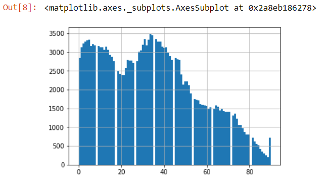
num_train['age'].hist(bins=100)

As we can see, the data set consists of people aged from 0 to 90 with the frequency of people declining with age. Using some intuition, it is highly unlikely the population below age 20 could earn >50K under normal circumstances. Therefore, we can bin this variable into age groups(covered in part 5. Data Manipulation).

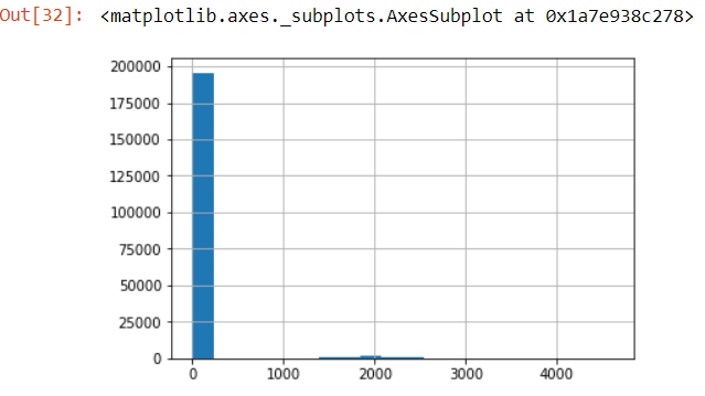
num_train['capital_losses'].hist(bins=20)

This is a nasty right skewed graph. In skewed distribution, normalizing is always an option. But we need to look into this variable deeper as this insight isn’t significant enough for decision making. One option could be to check for unique values. If they are less, we can tabulate the distribution (done in upcoming sections).

Furthermore, in classification problems, we should also plot numerical variables with dependent variable. This would help us determine the clusters (if exists) of classes 0 and 1. For this, we need to add the target variable in num_train data:

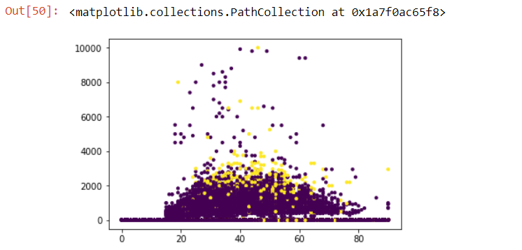
plt.scatter(num_train['age'], num_train['wage_per_hour'], c= cat_train['income_level'], s=10)

yellow scatter plots being those with income_level of binary value 1, and purple being those with income_level of binary value 0.

As we can see, most of the people having income_level 1, seem to fall in the age of 25-65 earning wage of $1000 to $4000 per hour. This plot further strengthens our assumption that age < 20 would have income_level 0, hence we will bin this variable.

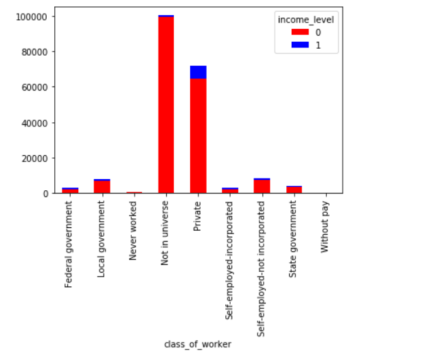
Similarly, we can visualize our categorical variables as well. Let’s do so for class_of_worker variable.

We can see that this variable looks imbalanced i.e. only two category levels seem to dominate. In such situation, a good practice is to combine levels having less than 5% frequency of the total category frequency (covered in part 5. Data Manipulation). The response Not in universe category appears unintuitive. Let’s assume that this response is given by people who got frustrated (due to any reason) while filling their census data.

Let’s visualize our education variable.

Evidently, all children have income_level 0. Also, we can infer than Bachelors degree holders have the largest proportion of people have income_level 1. Similarly, you can plot other categorical variables also.

4. Data Cleaning

Let’s check for missing values in numeric variables.

#Check for null values in our numerical columns
num_train.apply(lambda x: sum(x.isnull()),axis=0)

age 0
wage_per_hour 0
enrolled_in_edu_inst_lastwk 0
.
.

We see that numeric variables has no missing values. Good for us! Now, let’s check for missing values in categorical data.

#Check for null values in our numerical columns
num_train.apply(lambda x: sum(x.isnull()),axis=0)

class_of_worker 0
industry_code 0
.
.
migration_within_reg 99696
live_1_year_ago 0
migration_sunbelt 99696
country_father 6713
.
.
We find that some of the variables have ~50% missing values for cat_train; namely the migration columns. High proportion of missing value can be attributed to difficulty in data collection. For now, we’ll remove these category levels, for both train and test data.

cat_train = cat_train.drop(['migration_msa','migration_reg', 'migration_within_reg', 'migration_sunbelt'], axis = 1)
cat_test = cat_test.drop(['migration_msa','migration_reg', 'migration_within_reg', 'migration_sunbelt'], axis = 1)

For the rest of the missing values, a nicer approach would be to label them as ‘Unavailable’. Choosing the most suitable method for replacing missing values and imputing these values on large data sets can be painstakingly tedious.

cat_train = cat_train.fillna("Unavailable")

Let’s look at country_father, which previously had 6713 NA values, which should be labelled as Unavailable now.

cat_train['country_father'].value_counts()

United-States 159163
Mexico 10008
Unavailable 6713
Puerto-Rico 2680
.
.

5. Data Manipulation

We are approaching towards the machine learning stage. However machine learning algorithms return better accuracy when the data set has clear signals to offer. Specially, in the case of imbalanced classification, we should try our best to shape the data such that we can derive maximum information about the minority class.

In previous analysis, we saw that categorical variables have several levels with low frequencies(education in cat_train). Such levels don’t help as chances are they wouldn’t be available in test set. We’ll do this hygiene check in the coming steps.

Combining factor levels with low frequencies

In previous analysis, we saw that categorical variables have several levels with low frequencies(education in cat_train). Such levels don’t help as chances are they wouldn’t be available in test set. We’ll do this hygiene check in the coming steps.

cat_test['class_of_worker'].value_counts()

Not in universe 50079
Private 36071
Self-employed-not incorporated 4280
Local government 3833
State government 2167
Self-employed-incorporated 1648
Federal government 1405
Never worked 204
Without pay 75
Name: class_of_worker, dtype: int64

The code below combines categories in class_of_worker where they make up less than 5% of the total count. This should combine all categories with the exception of Not in universe and Private, and classify them as Other.

series = pd.value_counts(cat_train.class_of_worker)
mask = (series/series.sum() * 100).lt(5)
# To replace cat_train['class_of_worker'] use np.where. Example:
cat_train['class_of_worker'] = np.where(cat_train['class_of_worker'].isin(series[mask].index),'Other',cat_train['class_of_worker'])

cat_test['class_of_worker'].value_counts()

Not in universe 100245
Private 72028
Other 27250
Name: class_of_worker, dtype: int64

We do the same for cat_test as well. However do check if the proportion of class_of_worker is split evenly like cat_train as well.

series_test = pd.value_counts(cat_test.class_of_worker)
mask_test = (series_test/series_test.sum() * 100).lt(5)
# To replace cat_test['class_of_worker'] use np.where. Example:
cat_test['class_of_worker'] = np.where(cat_test['class_of_worker'].isin(series_test[mask_test].index),'Other',cat_test['class_of_worker'])

Not in universe 50079
Private 36071
Other 13612
Name: class_of_worker, dtype: int64

Binning numerical variables

Before proceeding to the modeling stage, let’s look at numeric variables and reflect on possible ways for binning. The specific variable we are interested in binning would be age; as seen previously where we plotted age against wage_per_hour colored by income level, with income level at binary value 0 for those 20 and under. There are various rule-of-thumbs to determine the binning range such as decision trees, I have included one such article here on deciding the binning range for variables.

We first define a function that allows us to easily bin variables:

#Binning:
def binning(col, cut_points, labels=None):
  #Define min and max values:
  minval = col.min()
  maxval = col.max()

  #create list by adding min and max to cut_points
  break_points = [minval] + cut_points + [maxval]

  #if no labels provided, use default labels 0 ... (n-1)
  if not labels:
    labels = range(len(cut_points)+1)

  #Binning using cut function of pandas
  colBin = pd.cut(col,bins=break_points,labels=labels,include_lowest=True)
  return colBin

And now we bin the age: 0-30 being renamed as young, 30-60 classified as adult, 60-90 classified as old. Let’s do this for our num_train dataframe first.

#Binning age
cut_points = [30,60]
labels = ["young","adult","old"]
num_train['age'] = binning(num_train['age'], cut_points, labels)

And now we bin our num_test dataframe.

cut_points = [30,60]
labels = ["young","adult","old"]
num_test['age'] = binning(num_test['age'], cut_points, labels)

Let’s verify to see if the column age in num_test dataframe is updated.

num_test['age']

0 adult
1 adult
2 young
3 adult
4 adult
.
.

Similarly, we should check on the other variables as well. For some of these variables, we are clear that more than 70-80% of the observations are 0. We can bin these variables as Zero and MorethanZero.

#Bin 'wage_per_hour' variable as 'Zero' and 'MorethanZero'
aa1 = num_train['wage_per_hour'] == 0
num_train['wage_per_hour'] = np.select([aa1], ['Zero'], default = 'MorethanZero')

num_train['wage_per_hour']

0 Zero
1 Zero
2 Zero
3 Zero
4 Zero
5 MorethanZero
.
.
We do this for num_test as well.

aa2 = num_test['wage_per_hour'] == 0
num_test['wage_per_hour'] = np.select([aa2], ['Zero'], default = 'MorethanZero')

Now, we can remove the dependent variable(income_level) from the training dataset (num_train).

# remove the dependent variable from num_train we added for visualization purpose earlier
num_train['income_level'] = 'NaN'

Let’s combine num_train and cat_train back to one training dataset, and num_test and cat_test back to one test dataset.

train_frames = [num_train, cat_train]
test_frames = [num_test, cat_test]
d_train = pd.concat(train_frames)
d_test = pd.concat(test_frames)

6. Machine Learning

Note: This portion is done in R and is largely inspired by Analytics Vidhya’s Imbalanced Dataset Project.

Making predictions on this data should atleast give us ~94% accuracy (due to our majority class forming roughly 94% of our data). However, while working on imbalanced problems, accuracy is considered to be a poor evaluation metrics because: 1.Accuracy is calculated by ratio of correct classifications / incorrect classifications.
2.This metric would largely tell us how accurate our predictions are on the majority class (since it comprises 94% of values). But, we need to know if we are predicting minority class correctly.
In such situations, we should use elements of a confusion matrix, to decide on the viability of a model.

We begin by importing our d_train and d_test into R, and making some minor adjustments before we use our model:

#load library for machine learning
> library(mlr)

#create task
> train.task <- makeClassifTask(data = d_train,target = "income_level")
> test.task <- makeClassifTask(data=d_test,target = "income_level")

The function ` makeClassifTask() in R helps us encapsulate the dataset by stating it as a classification problem, with the target variable we want to predict being income_level` as stated in the function above.

#remove zero variance features
> train.task <- removeConstantFeatures(train.task)
> test.task <- removeConstantFeatures(test.task)

Constant features can lead to errors in some models and obviously provide no information in the training set that can be learned from. The function removeConstantFeatures() in R helps us remove those variables with zero variance. #### Making our data balanced: Oversampling, Undersampling and SMOTE Now, we’ll try to make our data balanced using various techniques such as over sampling, undersampling and SMOTE. In SMOTE, the algorithm looks at the n-nearest neighbors, measures the distance between them and introduces a new observation at the center of n observations. While proceeding, we must keep in mind that these techniques have their own drawbacks such as:

• undersampling leads to loss of information
• oversampling leads to overestimation of minority class

We will try these 3 techniques and experience how it works.

#undersampling 
> train.under <- undersample(train.task,rate = 0.1) #keep only 10% of majority class
> table(getTaskTargets(train.under))

#oversampling
> train.over <- oversample(train.task,rate=15) #make minority class 15 times
> table(getTaskTargets(train.over))

#SMOTE
> train.smote <- smote(train.task,rate = 15,nn = 5)

Now that we have balanced our data using 3 separate techniques, let us see which algorithms are available for us to use. R has a neat function which lists the available algorithms we can use to solve a problem, by stating the type of problem (classification or regression) and how many classes our dependent variable takes (two in this case, 0 and 1 for income_level)

#lets see which algorithms are available
> listLearners("classif","twoclass")[c("class","package")]

One of the algorithms listed is Naive Bayes, an algorithms based on bayes theorem. We’ll use naive Bayes on all 4 data sets (imbalanced, oversample, undersample and SMOTE) and compare the prediction accuracy using cross validation.

#naive Bayes
> naive_learner <- makeLearner("classif.naiveBayes",predict.type = "response")
> naive_learner$par.vals <- list(laplace = 1)

#10fold CV - stratified
> folds <- makeResampleDesc("CV",iters=10,stratify = TRUE)

#cross validation function
> fun_cv <- function(a){
     crv_val <- resample(naive_learner,a,folds,measures = list(acc,tpr,tnr,fpr,fp,fn))
     crv_val$aggr
}

> fun_cv (train.task) 
# acc.test.mean tpr.test.mean tnr.test.mean fpr.test.mean 
# 0.7337249       0.8954134     0.7230270    0.2769730

> fun_cv(train.under) 
# acc.test.mean tpr.test.mean tnr.test.mean fpr.test.mean 
# 0.7637315      0.9126978     0.6651696     0.3348304

> fun_cv(train.over)
# acc.test.mean tpr.test.mean tnr.test.mean fpr.test.mean 
#   0.7861459     0.9145749     0.6586852    0.3413148

> fun_cv(train.smote)
# acc.test.mean tpr.test.mean tnr.test.mean fpr.test.mean 
#   0.8562135     0.9168955    0.8160638     0.1839362

This package names cross validated results as test.mean. After comparing, we see that train.smote gives the highest true positive rate and true negative rate. Hence, we learn that the SMOTE technique outperforms the other two sampling methods.

Now, let’s build our model SMOTE data and check our final prediction accuracy.

#train and predict
> nB_model <- train(naive_learner, train.smote)
> nB_predict <- predict(nB_model,test.task)

#evaluate
> nB_prediction <- nB_predict$data$response
> dCM <- confusionMatrix(d_test$income_level,nB_prediction)
# Accuracy : 0.8174
# Sensitivity : 0.9862
# Specificity : 0.2299

#calculate F measure
> precision <- dCM$byClass['Pos Pred Value']
> recall <- dCM$byClass['Sensitivity']

> f_measure <- 2*((precision*recall)/(precision+recall))
> f_measure 

The function confusionMatrix is taken from library(caret). This naive Bayes model predicts 98% of the majority class correctly, but disappoints at minority class prediction (~23%). Let’s use xgboost algorithm and try to improve our model. We’ll do 5 fold cross validation and 5 round random search for parameter tuning. Finally, we’ll build the model using the best tuned parameters.

#xgboost
> set.seed(2002)
> xgb_learner <- makeLearner("classif.xgboost",predict.type = "response")
> xgb_learner$par.vals <- list(
                      objective = "binary:logistic",
                      eval_metric = "error",
                      nrounds = 150,
                      print.every.n = 50
)

#define hyperparameters for tuning
> xg_ps <- makeParamSet( 
                makeIntegerParam("max_depth",lower=3,upper=10),
                makeNumericParam("lambda",lower=0.05,upper=0.5),
                makeNumericParam("eta", lower = 0.01, upper = 0.5),
                makeNumericParam("subsample", lower = 0.50, upper = 1),
                makeNumericParam("min_child_weight",lower=2,upper=10),
                makeNumericParam("colsample_bytree",lower = 0.50,upper = 0.80)
)

#define search function
> rancontrol <- makeTuneControlRandom(maxit = 5L) #do 5 iterations

#5 fold cross validation
> set_cv <- makeResampleDesc("CV",iters = 5L,stratify = TRUE)

#tune parameters
> xgb_tune <- tuneParams(learner = xgb_learner, task = train.task, resampling = set_cv, measures = list(acc,tpr,tnr,fpr,fp,fn), par.set = xg_ps, control = rancontrol)
# Tune result:
# Op. pars: max_depth=3; lambda=0.221; eta=0.161; subsample=0.698; min_child_weight=7.67; colsample_bytree=0.642
# acc.test.mean=0.948,tpr.test.mean=0.989,tnr.test.mean=0.324,fpr.test.mean=0.676

Now, we can use these parameters for modeling using xgb_tune$x which contains the best tuned parameters.

#set optimal parameters
> xgb_new <- setHyperPars(learner = xgb_learner, par.vals = xgb_tune$x)

#train model
> xgmodel <- train(xgb_new, train.task)

#test model
> predict.xg <- predict(xgmodel, test.task)

#make prediction
> xg_prediction <- predict.xg$data$response

#make confusion matrix
> xg_confused <- confusionMatrix(d_test$income_level,xg_prediction)
Accuracy : 0.948
Sensitivity : 0.9574
Specificity : 0.6585

> precision <- xg_confused$byClass['Pos Pred Value']
> recall <- xg_confused$byClass['Sensitivity']

> f_measure <- 2*((precision*recall)/(precision+recall))
> f_measure
#0.9726374 

As we can see, xgboost has outperformed naive Bayes model’s accuracy, with our F score(f_measure) being higher using xgboost. Having a specificity of 65%, this means for our model, 65% of the minority classes have been predicted correctly.

More measures can be taken to improve model accuracy, such as using only the important features instead of all the features (like what we are doing here), using the R function filterFeatures and doing XGboost on the model again. For now, I hope this model will suffice.